2.2 在一个种群中测量生物学衰老
Measurement of biological aging in an individual, although the most desirable and potentially the most accurate form of measurement, is highly variable and remains difficult to accomplish. Estimating the rate of aging in a population, by contrast, can be accomplished rather easily and has significantly less variability. However, population aging has less accuracy because, usually, the descriptor for the rate of aging is the change in mortality rate in the population with increasing age. Recall that aging and the risk of dying, although related, may not be the same, especially for species with a postreproductive life span. Moreover, an organism can die as a result of nonbiological aging events, such as trauma or disease, but its death will still be recorded in the dataset used in statistical calculations of the species' life span.
Do the problems associated with the use of mortality as a measure of aging in a population invalidate its use in the study of biological aging? Not by a long shot. Population mortality rates have been used for more than two hundred years in describing aging at the organismal level. Indeed, an analysis of mortality rates in the oldest cohort of a popuation has changed the way in which biogerontologists approach the study of aging and longevity (see the discussion at the end of this section). Many biogerontologists use the results from mortality analysis in a population to develop and test hypotheses that may predict individual aging or aging at the molecular level. Therefore, you need to have a basic understanding of the derivation, use, and limitations of mortality rate in describing aging within a population.
2.2.1 Mortality rates estimate the number of deaths in populations
Determining the crude mortality, the death rate in a total population without regard to age, is fairly simple, provided one has an accurate count of the population size and the number of deaths (Equation 2.1).
This mortality rate, M, is normally converted to a standard measure—for example, deaths per 1000 or 100,000 individuals per year—for ease of interpretation and comparison.
Measuring the number of deaths in a human population in most countries poses few problems, because law requires formal recordings of deaths. However, the size of the population at any given time can only be estimated, using data derived from the most recent census. In the United States, a population census is conducted every 10 years. To reduce error associated with estimating the actual size of a population, human mortality rates are calculated as statistical probabilities by using actual death rates applied to a hypothetical population size, such as 100,000. Although human mortality rates are considered estimates, they have been shown to be extremely precise and should be considered accurate descriptions of the death rate in a population.
Mortality rates can be determined for nonhuman populations as well. Measurements of population size and number of deaths in short-lived species monitored under laboratory conditions can be extremely precise, and, thus, so are the mortality rates. However, population size and deaths are difficult to measure in long-lived wild populations. Imagine trying to count the population size and deaths of a particular bat species (bats can live up to 20 years) living in the United States—an impossible task. Therefore, wildlife demographers typically confine their work to small areas, say 2–3 acres, housing a high-density population, then extrapolate the mortality rate to the general population.
2.2.2 Life tables contain information on mortality, life expectancy, and the probability of dying
A life table describes the death characteristics of a population at specific ages or age intervals. There are two types of life tables. A cohort life table follows the death characteristics of a population of a single birth cohort that can be observed throughout the life span. The cohort life table is useful for species having short life spans or for historical populations having accurate birth and death records. Following a live birth cohort in long-lived species, including humans, throughout the actual life span is not practical. In these cases, the current or period life table is used. A current life table applies the current death characteristics of a living population to a hypothetical birth cohort, usually 100,000 (TABLE 2.2) . These values are then used to forecast mortality statistics over the life span of an actual population, based on data collected at a single time point. In either case, cohort or current life table, the mechanics of constructing the values given in the life table are the same. Life tables can be either complete or abridged. A complete life table is defined as one in which the age interval is one year. Use of all other age groupings defines an abridged life table—such as the life table presented in Table 2.2.
TABLE 2.2 ABRIDGED LIFE TABLE FOR THE TOTAL UNITED STATES POPULATION, 2006
Life tables, cohort or current, consist of seven columns. Because a life table is used throughout the world as the primary mechanism to estimate the rate of death in a population, the column names and variable designations are standardized by convention. Column 1 contains the age (in the case of a complete life table) or age interval (in the case of an abridged life table). With the exception of the first age interval in a human life table, in which the interval 0–1 years must be used, the selection of the age or age interval is at the discretion of the statistician constructing the table; with human data, it is customary to use 5-year intervals for an abridged table. Column 2 contains the probability of death (q x ), also known as age-specific mortality. Column 3 shows the number of persons from the original 100,000 of the hypothetical cohort who are alive at the beginning of the age interval (l x ). Column 4 shows the number dying (d x ) for each interval. Column 5, person-years lived (L x ), represents the total time (in years) lived between two birthdays for he population at each age interval. Column 6 contains the total number of person-years that would be lived (T x ) after the beginning of the age interval x to x+ n. Finally, Column 7 gives the life expectancy (e x ). The life expectancy is the average number of years remaining to be lived by those surviving to that age.
The information contained in the life table is the primary tool of the demographer and has many uses for the trained specialists, uses that are well beyond the scope of this text. Here, we are concerned primarily with how the rates of mortality, primarily q x , and the shape of the curves derived from the calculation of mortality rate help to describe aging in a population. The Appendix contains a more detailed description of how a life table is constructed, including more precise definitions and the method of calculating each variable.
2.2.3 Age-specific mortality rate rises exponentially
The age-specific mortality rate (qx) is a useful measurement in aging research (Equation 2.2). It is calculated as follows:
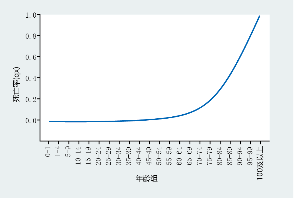
Age-specific mortality rate simply describes the chance (probability) of dying within a specific age range. For example, Table 2.2 shows a q x value of 0.011 for the age interval 40–44 years. This means that you have a 1.1% chance of dying during this age interval. Graphing the age specific mortality allows us to visualize the rate over a lifetime. As you can see in Figure 2.11, the probability of death between ages 1 and 70 increases slowly. After age 70, age-specific mortality increases and continues to increase at an apparently constant rate until the entire population has died.
Figure 2.11 Age-specific mortality rate, q x , for the total United States population, 2006. (Data from E. Arias, United States life tables, 2006, Natl Vital Stat. Rep. 58:1-40, 2010. With permission from the National Center for Health Statistics.)
The shape of the age-specific mortality graph suggests an exponential function. Benjamin Gompertz noted this in 1825 and suggested that age-specific mortality rate accelerates in populations that have a significant number of individuals that survive to the age of reproduction. Thus, the function that describes the rate of mortality in a population bears his name: the Gompertz mortality function (Equation 2.3) .
This function can be rewritten algebraically:
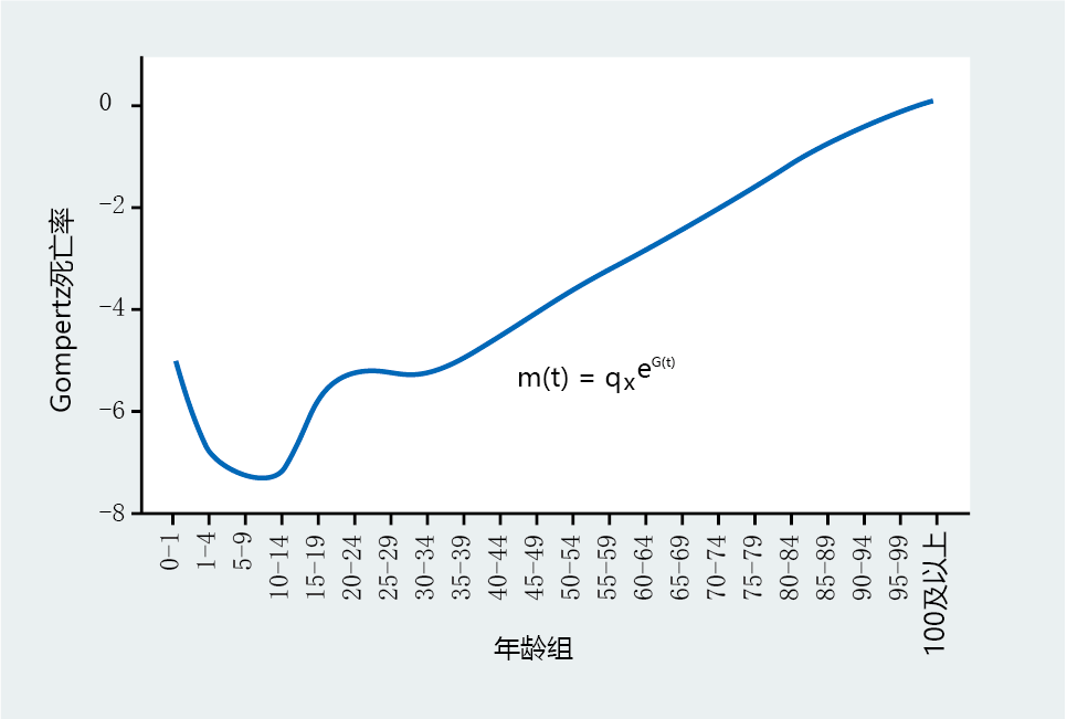
As shown in Figure 2.12, the Gompertz mortality rate describes a constant increase in mortality with age, thus providing a marker of biological aging in the postdevelopment population. Note that the mortality rate of the age interval 0–1 years does not conform to the exponential increase characterizing the other age groups. In a human population, the death rate of individuals from birth to 1 year of age defines the infant mortality rate and will always be significantly higher than that of other childhood intervals, due to the inherent risk of birth and infancy. The impact of the infant mortality rate on aging is discussed in later chapters. Also note the slight rise in mortality that occurs around the ages of 10–15 and 15–20. Gerontologists refer to this rise as the “I-think-I-am-immortal” effect, because of the propensity of males to engage in risky behaviors that cause death. It is also known as the “stupidity or testosterone bump.”
Figure 2.12 Gompertz mortality rate, m ( t ), for the total United States population, 2006. (Data from E. Arias, United States life tables, 2006, Natl Vital Stat. Rep. 58:1–40, 2010. With permission from the National Center for Health Statistics.)
2.2.4 Age-independent mortality can affect the mortality rate
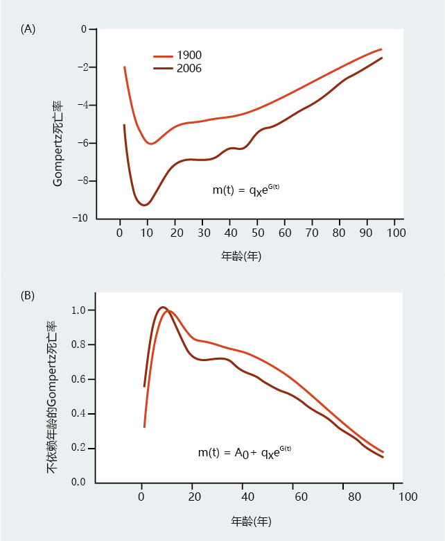
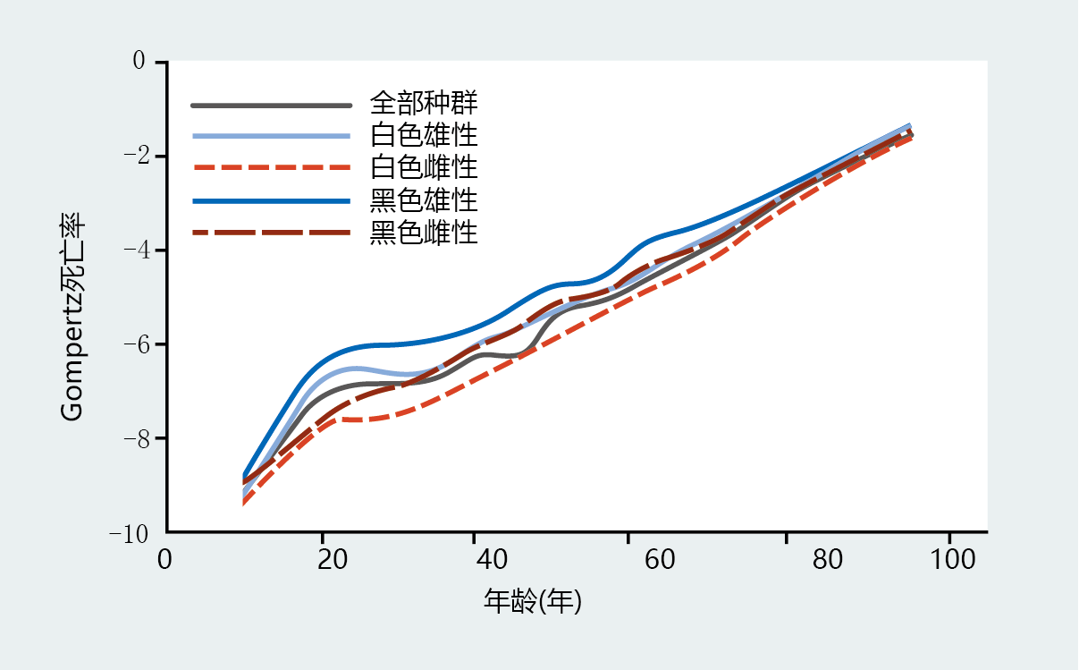
Gompertz assumed that all members of the population, even the very young, died of natural causes due to age-dependent mortality, or biological aging. However, death can occur as a result of accidents or other 环境ally induced trauma, such as infections, that do not reflect biological aging. Moreover, current understanding of age-dependent mortality does not, for the most part, include deaths before puberty. Death that is not the result of biological aging is known as age-independent mortality and can be included as a variable in the Gompertz mortality function. Generally, age-independent mortality is included in the Gompertz mortality function equation only when comparing the mortality rates of different populations of a species that have significantly different 环境al influences on death—war, infectious disease, and so on (Figure 2.13) . In addition, most research has shown that age-independent mortality varies considerably before puberty and then becomes constant in stable populations that are not exposed to excessive 环境al insults (Figure 2.14) . Therefore, calculation of the Gompertz mortality function (Equation 2.3) will not generally include data for age-specific mortality before puberty. In other words, calculation of the function begins with data at the lowest mortality rate, usually around the time of puberty.
Figure 2.13 Comparison of the Gompertz mortality function and the age-independent Gompertz mortality function. These graphs show the mortality rates in the United States in 1900 and 2006 by graphing (A) the standard Gompertz mortality function and (B) the standard Gompertz mortality with a constant, A 0 , added to account for ageindependent mortality (the lowest mortality rate for each population was used as age-independent mortality). Note that the differences in early life mortality shown in (A) are partially eliminated by correcting for agendependent mortality. (Data from F.C. Bell and M.L. Miller, Life Tables for the United States Social Security Area 1900–2010, Pub. No. 11-11536, Washington, DC: Social Security Administration, 2005; data from E. Arias, United States life tables, 2006, Natl Vital Stat. Rep. 58:1–40, 2010. With permission from the National Center for Health Statistics.)
Figure 2.14 Gompertz mortality plots for different United States populations, 2006. The lowest mortality rate in all groups occurs around the age of 10 years. Although mortality rates for the four populations differ during young adulthood, the mortality rates after age 40 are similar. (Data from E. Arias, United States life tables, 2006, Natl Vital Stat. Rep. 58:1–40, 2010. With permission from the National Center for Health Statistics.)
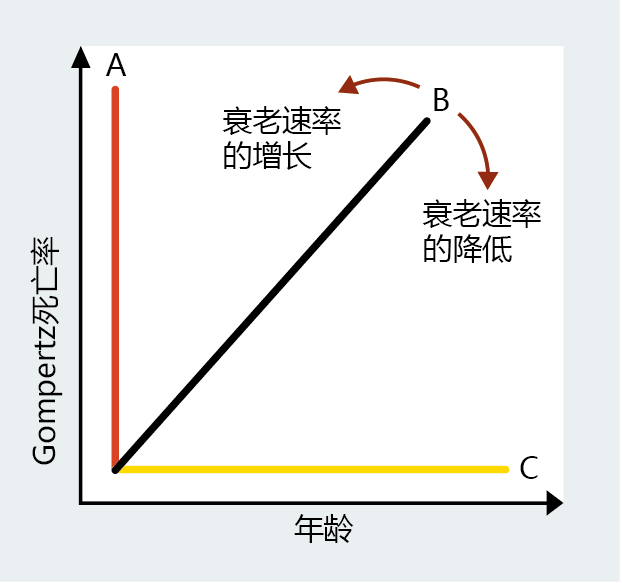
Because age-dependent and age-independent mortality have been defined and can be dealt with mathematically, we now have a method for evaluating the rate of aging by using the Gompertz mortality function between or within populations of the same species that may or may not be experiencing different conditions—socioeconomic status, cure or treatment of a disease, pollution, and so forth. Many statistical techniques are used in the science of demography to make comparisons in mortality rates between different populations. For the purpose of this text, visually examining the slope of the lines generated by the Gompertz mortality function provides an easy method to determine possible changes in the rate of aging. For example, the hypothetical Gompertz plots shown in Figure 2.15 illustrate three different rates of aging based on mortality rate analysis. Line A is indicative of populations that age very rapidly. Line B approximates the Gompertz function of a population in which aging is gradual. The flat line C, slope = 0, characterizes populations that do not appear to undergo aging. Now consider a population in which the rate of aging can be described by line B. If we introduce a cure for, say, lung cancer into the population, after an appropriate amount of time we can measure the rate of aging again using Gompertz analysis. If line B changes in the direction of line C, then we can conclude that we have slowed the rate of aging in the population by treating lung cancer. If the line shifts toward line A, then we can conclude that curing lung cancer has increased the rate of aging.
Figure 2.15 A change in slope of the Gompertz mortality rate provides a measure of change in the rate of aging in a population. As the slope moves toward line A, the rate of aging increases. As the slope moves toward line C, the rate of aging decreases
2.2.5 Mortality-rate doubling time corrects for differences in initial mortality rates
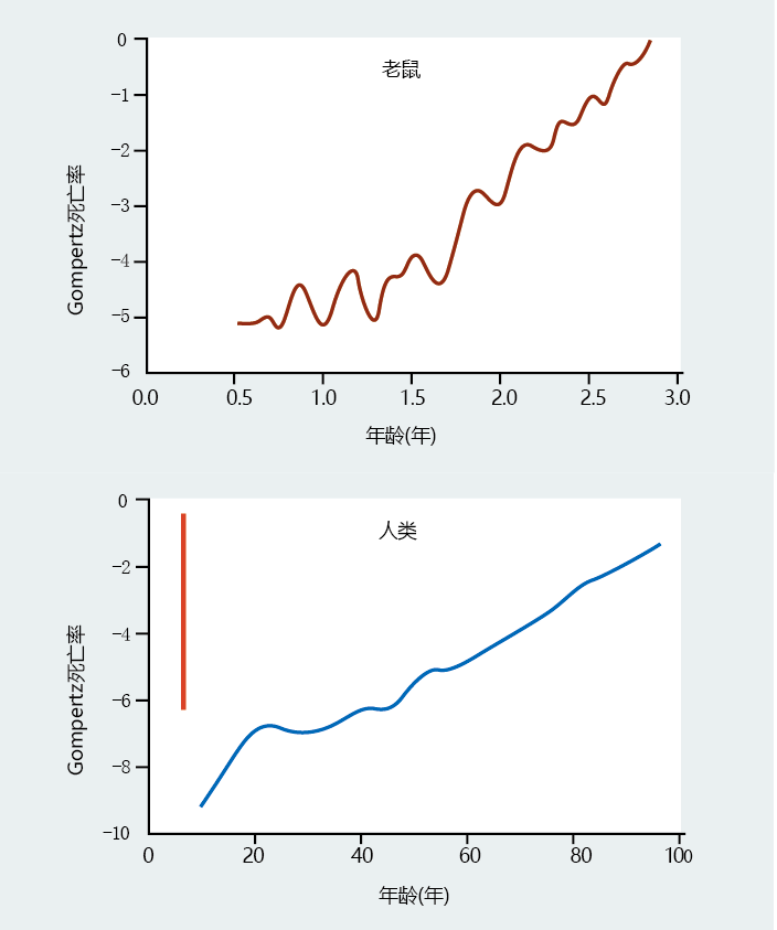
Using the Gompertz analysis for measuring the rate of aging in populations of a single species has proved very useful to biogerontologists. However, comparisons between the rates of aging of different species, while possible with Gompertz analysis, can be difficult to interpret, because population size, age-independent mortality, and maximum life span vary widely among species (Figure 2.16) . While some demographers have developed sophisticated mathematical schemes to account for these differences, such procedures include many assumptions and
techniques that are not easily applied to all species. Dr Calab Finch suggested in 1990 that the difficulties associated with using Gompertz analysis for comparisons between species could be partially reduced by the simple calculation of the mortality-rate doubling time (MRDT), or the time required for the mortality rate in a population to double, given by Equation 2.5.
Figure 2.16 Comparison of Gompertz mortality rates of two different species. These graphs show the Gompertz mortality plots for a population of mice and for the total United States population in 2006. Although the small size of the mouse population causes significant variation in the data, note that the pattern of mortality after a specific age (1.5 years in the mice, 25 –30 years in the humans) is similar and describes a gradual rate of aging. However, differences in age-independent mortality and maximum life span can be difficult to compare between species. If we were to plot the mouse data on the same x-axis scale as the human data, the result would be the red line on the human plot. (Bottom data from E. Arias, United States life tables, 2006, Natl Vital Stat. Rep. 58:1–40, 2010. With permission from the National Center for Health Statistics.)
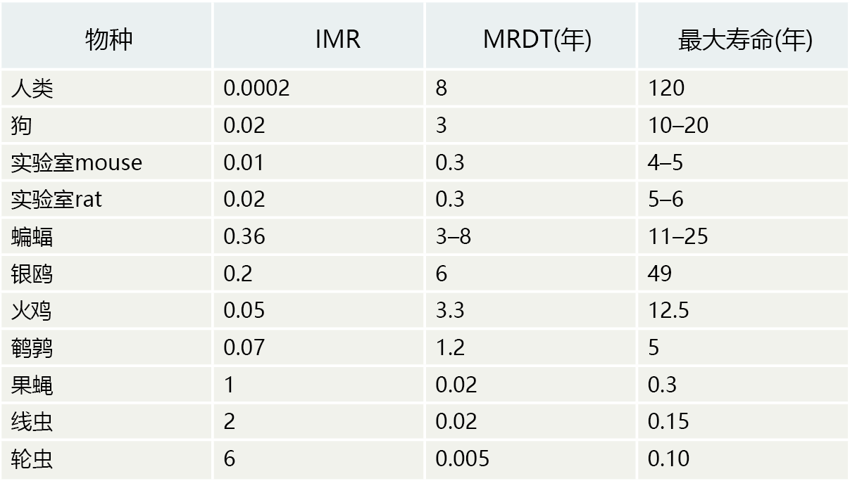
Analysis of the rate of aging that includes the MRDT often forms the basis for testing hypotheses about the individual rate of aging. For example, consider the data for the human, dog, and bat in TABLE 2.3 . The initial mortality rate (IMR) tells us that humans have become extremely good at limiting mortality in the early years of life. Bats, because they are wild animals, are not as good as humans at protecting their young, as indicated by the higher IMR. Moreover, the bats‘ maximum life span is only about 20% that of humans. If we had only these two variables as our markers for the rate of aging in a population, one logical conclusion would be that IMR significantly affects maximum life span. Note, however, that the domestic dog has an IMR somewhere between that of the human and the bat, but a maximum life span equal to that of the bat. Therefore, it is unlikely that IMR determines life span. We must find another answer for why maximum life spans differ among species.
TABLE 2.3 INITIAL MORTALITY RATE (IMR), MORTALITY-RATE DOUBLING TIME (MRDT), AND MAXIMUM LIFE SPAN OF VARIOUS SPECIES
Addition of the MRDT to the analysis gives some insight on what might be happening.
Although bats have a high IMR, their average MRDT of 5 years suggests a slower aging rate than that observed in domesticated dogs, which have an MRDT of 3 years. We must consider, however, that domesticated dogs often receive several of the health care benefits that are afforded humans. This would, in all likelihood, contribute to the dogs' long lives by reducing age-independent mortality. Bats are wild and thus tend to have a rather short postreproductive life span, due to predation and diseases. In other words, compared with dogs, bats have high ageindependent mortality. Nonetheless, the MRDT of 5 years suggests that bats have a rate of aging much closer to that of humans than dogs do. The MRDT of bats is also significantly greater than that observed in mice and rats, the two most common species used in aging research. Given appropriate 环境al conditions that would help to reduce age-independent mortality, the bat would make a good model for the human for evaluating possible factors that influence the individual rate of aging. Indeed, many laboratories are breeding bats in captivity for this very purpose.
2.2.6 Survival curves approximate mortality rate
The construction of a life table and analysis of mortality rates are time-consuming and generally complicated. Moreover, an accurate determination of mortality rates requires large population samples, a luxury that most biologists do not have. Therefore, biogerontologists use the simpler survival curve, a graphical representation of survival over time, to estimate the rate of aging in a population (Figure 2.17)
Figure 2.17 Comparison of survival curves for two different species. Survival curves are generated from a life table (see Table 2.2). Column 1 (age) is plotted against the conversion of column 3 (l x ) to percentage of life span. The patterns of survival for the mouse population and for the human population in 2006 are similar, suggesting that survival curves in a small population are a good approximation of true mortality rates. (Bottom data from E. Arias, United States life tables, 2006, Natl Vital Stat. Rep. 58:1–40, 2010. With permission from the National Center for Health Statistics.)
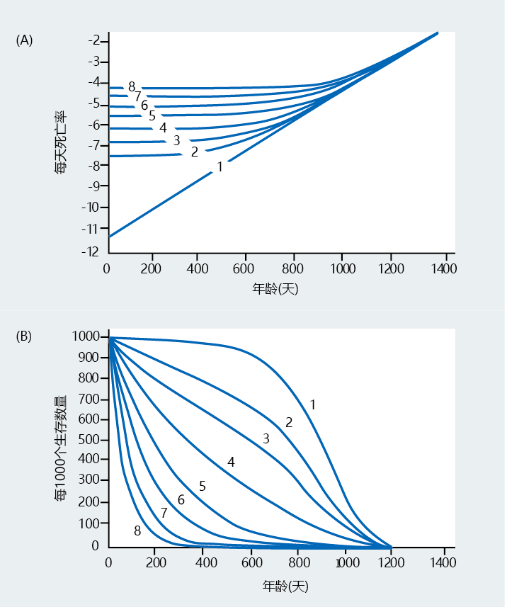
The same general assumptions concerning the rate of aging that are applied to the life table can be used for the survival curve. Indeed, comparing the shape of the survival curve with the log of mortality rate demonstrates that as the nature of mortality changes, so too does the shape of the survival curve (Figure 2.18).
Figure 2.18 Comparison of Gompertz mortality rate plots and survival curves. (A) Gompertz plot. (B) Survival curve. Numbers on the lines indicate the same populations in both graphs. For example, line 1 in (A), the mortality rate expected for a gradually aging population, corresponds to line 1 in (B), the expected survival curve for the same population. As the pattern of the Gompertz mortality rate changes, so does the pattern for survival, indicating that survival curves are a good approximation of mortality rate. (From G.A. Sacher, in Handbook of the Biology of Aging [C.E. Finch and L. Hayflick, eds.], New York: Van Nostrand Reinhold Company, 1977. With permission from John Wiley and Sons)
The data used to construct a survival curve also provide two important variables—mean life span and maximum life span—that are used extensively in biogerontology. Mean life span corresponds to the arithmetic average of the life span in the population. Maximum life span reflects the age of death of the longest-lived individual in the population. Biogerontologists often use the upper 10% of survival as their marker of maximum life span because survival curves are normally generated from numerically small populations and few individuals reach very old age. Both mean life span and maximum life span have specific meanings with regard to factors affecting the shape of the survival curve. Mean life span is a measure of extrinsic aging in populations.
Biogerontologists compare mean life spans of populations of a single species that are exposed to different 环境s or experimental treatments to determine whether external factors affect the rate of population senescence. Note that deaths in the first 50% of the populations described in Figure 2.17 occur over a long period of time. On the other hand, the second 50% of the populations die within a short percentage of the life span. Thus, mean life span is a relative measure of the survival rate during development and maturity phases and the impact of these two life phases on senescence. Note how the change in early life survival of the human population shown in Figure 2.17 changes the mean life span. A positive change in mean life span would suggest that some external intervention slowed the extrinsic rate of aging and allowed a greater proportion of the population to enter senescence. Conversely, a negative change in mean life span denotes an increase in the extrinsic rate of aging and fewer individuals that will senesce. The fewer the individuals reaching senescence, the greater the likelihood that any conclusion made concerning maximum life span may be influenced by selective mortality.
Maximum life span provides the biogerontologist with some information about the genetic or intrinsic rate of aging. You will learn in the coming chapters that life span potential has evolved from genes selected for successful reproduction, although those genes have not yet been identified. Thus, any change in maximum life span following some treatment or experimental procedure can be taken to mean that
some fundamental property of intrinsic aging, most likely genetic, has been altered. Notice that the maximum life spans of the three human populations in Figure 2.17 are identical, even though the shapes of the survival curves are different. That is, maximum life span was not affected by the extrinsic rate of aging.
2.2.7 Deceleration of mortality rate at the end of life suggests the possibility of 寿命 genes
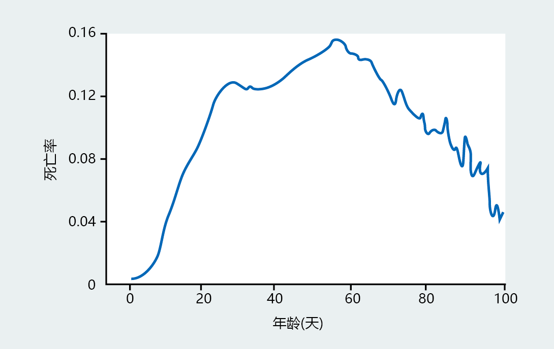
Close inspection of the survival curves in Figure 2.17 suggests that the rate of survival increases slightly toward the end of the life span for these populations. The change in rate at the tail of survival curves is a common observation and suggests that the late-life mortality rate may slow rather than remain constant as predicted by Gompertz. Several researchers have investigated this possibility and found a deceleration in mortality rate in late life, when the populations studied have sufficient numbers of individuals left at the end of life to allow accurate analysis. The first to recognize this phenomenon was Dr. James Carey at the University of California, Davis. He used more than 1.2 million Mediterranean fruit flies to demonstrate that mortality rate declines in flies in old age (Figure 2.19). The implications of these findings are that the Gompertz mortality function does not accurately describe the trajectory of mortality at all stages of life and that one cannot predict, with accuracy, the maximum life span for a population.
Figure 2.19 The mortality rate for 1.2 million fruit flies. From 0 to 20–30 days of age, the rate shows the typical exponential increase expected for a population kept under laboratory conditions—that is, little age-independent mortality. However, the analysis of this large population of fruit flies shows that mortality slows and decelerates in late life, unlike the constant mortality rate predicted by Gompertz. (From J.R. Carey, P. Liedo and J.W. Vaupel, Exp. Gerontol. 30:605–629, 1995. With permission from Elsevier.)
Since immortality has not been observed in any species known to senesce, does the finding that maximum life span may not be fixed have practical applications? Most likely not. But deceleration of late-life mortality has huge theoretical implications for biogerontological investigators who study the 进化 and genetics of aging. As you will learn in the next chapter, 进化ary theory predicts that longevity has arisen from genes selected for successful reproduction; that is, genes determine longevity. The data in fruit flies are consistent with 进化ary theory and show that a subset of the population has different longevity characteristics than the majority of the population. Since longevity is determined by the genome, it follows that this subset of fruit flies must have different genes that allow them to live longer and to senesce at a different rate. The work in fruit flies provides the theoretical basis that molecular biologists and geneticists are using to test hypotheses about possible candidate genes that modify life span.
ESSENTIAL CONCEPTS
- Biogerontologists have traditionally used the passage of time as the standard unit of measurement for expressing age-related change. However, trying to determine whether possible timerelated differences seen at the chosen time points have any meaning for biological aging can be difficult and often leaves many unanswered questions.
- Due to differences in our interactions with the 环境, the rate of biological aging is highly individualized.
- The intrinsic rate of aging reflects an individual‘s genotype and can be measured with a fair amount of accuracy. The extrinsic rate of aging, a result of the 环境‘s interaction with the genotype—that is, the phenotype—has infinite possibilities and can be challenging to measure.
- Regulation of gene expression that results in the phenotype can also be influenced by epigenetic effects.
- Differences between the phenotypes of individuals increase with age. As we grow older, the phenotype becomes more and more unique to the individual.
- Recent research has suggested that the trajectory in the rate of aging may be established during fetal and early life development.
- Cross-sectional investigations compare the means of different age groups at a single point in time. Cross-sectional studies have limited precision, due to factors such as intrinsic variability, the cohort effect, and selective mortality.
- Longitudinal studies have shown that the rate and timing of age-related physiological functional decline are highly variable. Longitudinal studies have also shown that age-related physiological decline is nonlinear with respect to time.
- Personal genomics may soon be used to identify whether “rate of aging” genes exist and how these genes are expressed.
- Biogerontologists can estimate the rate of aging in a particular population by calculating mortality rates.
- Data from life tables can approximate both the current probability of dying, or age-specific death rate (q x ), and the life expectancy of an individual (e x ).
- The Gompertz mortality function, m(t) = q x e G(t) , describes the rate of mortality in a population.
- Comparison of mortality rates between populations having different 环境al conditions that affect mortality must include a measure of age-independent mortality.
- Difficulties associated with using Gompertz analysis for comparisons between species, due to differences in population size, initial mortality rate, and maximum life span, can be partially reduced by calculating the mortality-rate doubling time, MRDT = ln 2 /G.
- Survival curves are graphical representations of survival over time and can be used to estimate the rate of aging in a population when construction of life tables and analysis of mortality rates are impractical.
- Current data indicate that the rate of survival increases slightly toward the end of the life span in many populations, suggesting that the late-life mortality rate may slow.


